Quick Guide-Part 2

In the first part of this tutorial, we talked about three modules (structdata, feature_engineering, timeseries) modules available in datasist. In this post, we'll cover the visualization and model modules. So without further ado, let's get to it.

What you will learn in this part:

Easy visualization with the visualization module.
- Visualization for categorical features.
- Visualization for numerical features.
Machine learning with the model module.

Before we begin, let's import the data set and libraries we will use for this analysis. If you're just joining us here, please read Part 1 so we can be on the same page.

We are using the same dataset from the last part. Download the dataset from here

import pandas as pd
import datasist as ds
import numpy as np

train_df = pd.read_csv('train_data.csv')
train_df.head()

Output:

	Customer Id	YearOfObservation	Insured_Period	Residential	Building_Painted	Building_Fenced	Garden	Settlement	Building Dimension	Building_Type	Date_of_Occupancy	NumberOfWindows	Geo_Code	Claim
0	H14663	2013	1.0	0	N	V	V	U	290.0	1	1960.0	.	1053	0
1	H2037	2015	1.0	0	V	N	O	R	490.0	1	1850.0	4	1053	0
2	H3802	2014	1.0	0	N	V	V	U	595.0	1	1960.0	.	1053	0
3	H3834	2013	1.0	0	V	V	V	U	2840.0	1	1960.0	.	1053	0
4	H5053	2014	1.0	0	V	N	O	R	680.0	1	1800.0	3	1053	0

Easy visualization using datasist.

The visualization module is one of the strong areas of datasist. There are numerous functions available for creating aesthetic and colorful plots with minimal code. In this post, we'll highlight some of the functions available.

All functions in the visualization module works at data scale not feature scale. This means, you can visualize a full dataset in one go. You can also specify individual features you want to plot.

Visualization for Categorical features

Visualization for categorical features include plots like boxplot, violinplot, countplots etc. We can use the functions available in datasist to easily do this at data wide level. Some of the functions are:

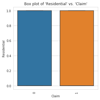
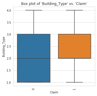
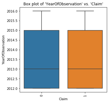
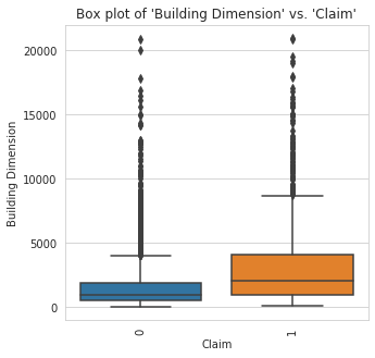
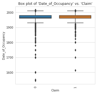
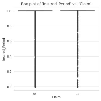
boxplot: This function makes a box plot of all numerical features against a specified categorical target column.

TLDR;

A box plot (or box-and-whisker plot) shows the distribution of quantitative data in a way that facilitates comparisons between variables or across levels of a categorical variable. The box shows the quartiles of the dataset while the whiskers extend to show the rest of the distribution, except for points that are determined to be "outliers" using a method that is a function of the inter-quartile range.

You can save a plot as a png file in the current folder by setting the save_fig parameter to True in any of the visualization function

ds.visualizations.boxplot(train_df, target='Claim')

Output:

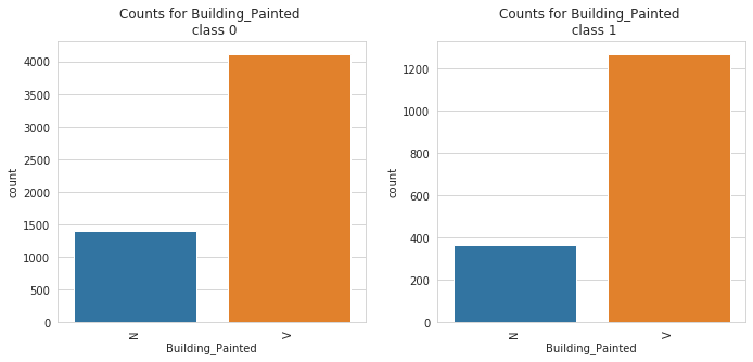
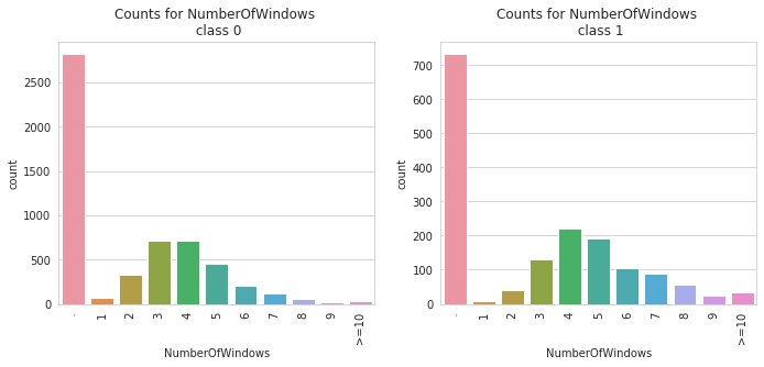
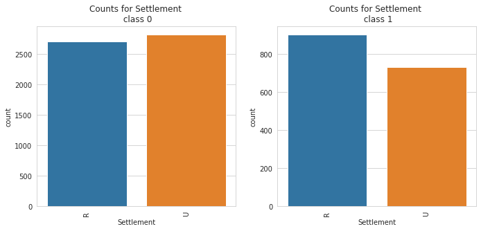
2. catbox: The catbox is used to make a side by side bar plot of all categorical features in a dataset against a specified categorical target. This can help in identifying causation and patterns and also identifying features that help separates a specified target.

catbox can only plot categorical feature with a limited number of unique classes. Also, the target must be a categorical feature with a limited number of unique classes as well.

ds.visualizations.catbox(train_df, target='Claim')

Customer Id feature has too many categories and will not be plotted
Geo_Code feature has too many categories and will not be plotted

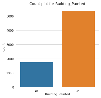
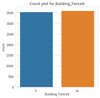
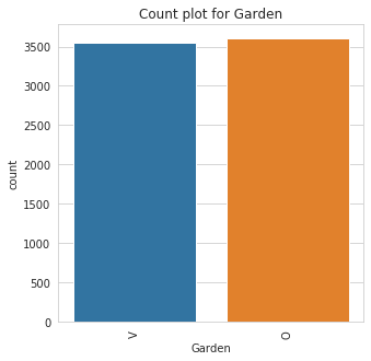
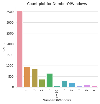
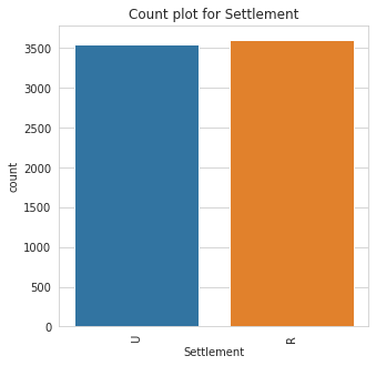
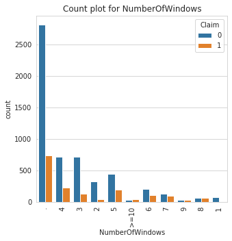
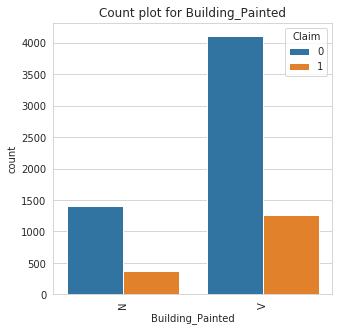
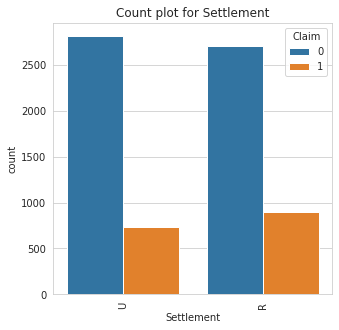
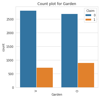
3. countplot: The countplot makes a barplot of all categorical feature to show their class count.

You can specify specific features to plot else, it is automatically inferred. You can also choose to separate by specific feature

ds.visualizations.countplot(train_df)

Unique Values in Customer Id is too large to plot
Unique Values in Geo_Code is too large to plot

ds.visualizations.countplot(train_df, separate_by='Claim')

Unique Values in Customer Id is too large to plot
Unique Values in Geo_Code is too large to plot

Visualization for Numerical features

Visualization for numerical features include plots like scatterplot, histogram, kde plots etc. Let's understand some of these functions below:

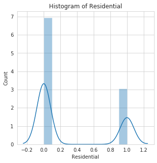
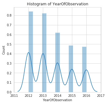
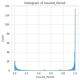
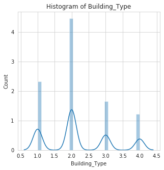
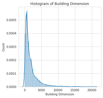
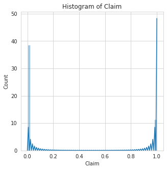
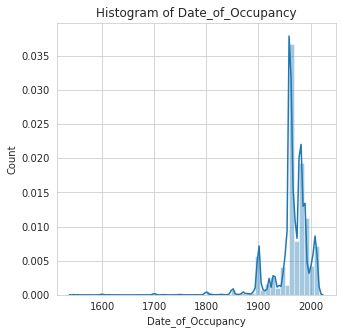
histogram: This function makes an histogram plot of all numerical features in a dataset. This Helps to show distribution of the features.

To use the histogram function, the specified features to plot must not contain missing values, else it would throw an error.

In the example below, the features Building Dimension and Date_of_Occupancy both contain missing values. We can decide to fill them before plotting or we could pass in a list with these features removed.

we'll go with the first option, that is filling the missing values using the fill_missing_num function of datasist before plotting.

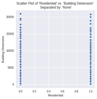
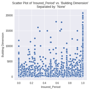
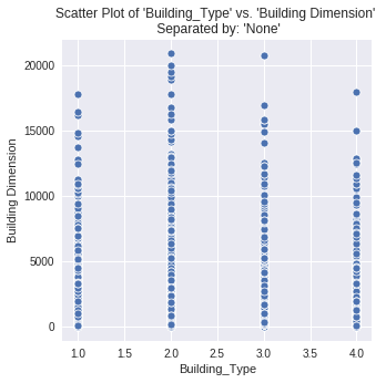
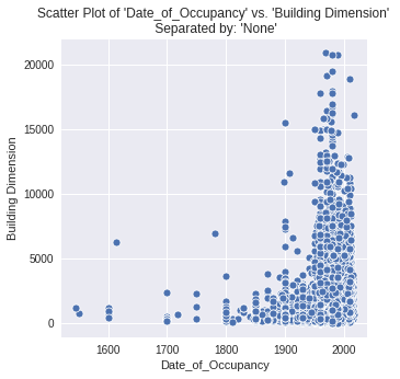
df = ds.feature_engineering.fill_missing_num(train_df)
ds.visualizations.histogram(df)

****

2. scatterplot: This function makes a scatter plot of all numerical features in a dataset against a specified **numerical target. It helps to show the correlation between features.

feats = ['Insured_Period',
         'Residential',
         'Building Dimension',
         'Building_Type',
         'Date_of_Occupancy']

ds.visualizations.scatterplot(train_df,num_features=feats, target='Building Dimension')

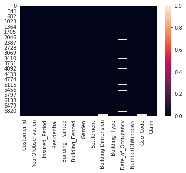
3. plot_missing: As the name implies, this function can be used to visualize the missing values in a dataset. White cells indicate missing and dark cells indicate not-missing. The color range at the right hand corner shows intensity values.

ds.visualizations.plot_missing(train_df)

Isn't It amazing how you can get things done quickly with just a line of code in datasist? It sure is!

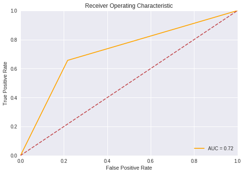
The goal is to make data analysis quicker and easier. Other functions available in the visualization module are plot_auc, plot_confusion_matrix, violin_plot etc. Read more about these functions here.

Machine learning with the model module

The model module contains functions and methods for testing and comparing machine learning models. Current version of datasist only supports sci-kit learn models. Tensorflow and Pytorch models will be supported soon. we'll highlight some of the important functions in this model below.

To demonstrate these functions, we'll use the dataset available here. The task is to predict insurance claim (1=Claim, 0=No Claim) from building observations. In other to demonstrate using the model module, we'll do some basic data processing first.

The goal of this analysis is to demonstrate how to use the model module, so we would not be doing any heavy feature engineering.

import pandas as pd
import numpy as np
import datasist as ds

pd.set_option('display.max_colwidth', 400)


train = pd.read_csv('train_data.csv')
test = pd.read_csv('test_data.csv')
vardef = pd.read_csv("variabledef.csv")

Let's display the variable definitions to better understand the data

vardef

Variable

Description

Customer Id

Identification number for the Policy holder

YearOfObservation

year of observation for the insured policy

Insured_Period

duration of insurance policy in Olusola Insurance. (Ex: Full year insurance, Policy Duration = 1; 6 months = 0.5

Residential

is the building a residential building or not

Building_Painted

is the building painted or not (N-Painted, V-Not Painted)

Building_Fenced

is the building fence or not (N-Fenced, V-Not Fenced)

Garden

building has garden or not (V-has garden; O-no garden)

Settlement

Area where the building is located. (R- rural area; U- urban area)

Building Dimension

Size of the insured building in m2

Building_Type

The type of building (Type 1, 2, 3, 4)

Date_of_Occupancy

date building was first occupied

NumberOfWindows

number of windows in the building

Geo Code

Geographical Code of the Insured building

Claim

target variable. (0: no claim, 1: at least one claim over insured period).

#drop the id column
train.drop(columns='Customer Id', axis=1, inplace=True)
test.drop(columns='Customer Id', axis=1, inplace=True)

#fill missing values
train = ds.feature_engineering.fill_missing_cats(train)
train = ds.feature_engineering.fill_missing_num(train, method='mean')

test = ds.feature_engineering.fill_missing_cats(test)
test = ds.feature_engineering.fill_missing_num(test, method='mean')

ds.structdata.display_missing(train)

	features	missing_counts	missing_percent
0	YearOfObservation	0	0.0
1	Insured_Period	0	0.0
2	Residential	0	0.0
3	Building_Painted	0	0.0
4	Building_Fenced	0	0.0
5	Garden	0	0.0
6	Settlement	0	0.0
7	Building Dimension	0	0.0
8	Building_Type	0	0.0
9	Date_of_Occupancy	0	0.0
10	NumberOfWindows	0	0.0
11	Geo_Code	0	0.0
12	Claim	0	0.0

Now that we have successfully filled all missing values in the dataset, we'll encode all categorical features using either label encoding, or one hot encoding depending on the number of unique classes.

#check the unique classes in each categorical feature
ds.structdata.class_count(train)

Class Count for Building_Painted

Building_Painted

5382

1778

Class Count for Building_Fenced

Building_Fenced

3608

3552

Class Count for Garden

Garden

3609

3551

Class Count for Settlement

Settlement

3610

3550

Class Count for NumberOfWindows

	NumberOfWindows
.	3551
4	939
3	844
5	639
2	363
6	306
7	211
8	116
1	75
>=10	67
9	49

Unique classes in Geo_Code too large

We will label encode Geo_Code, since the unique classes is large, and one-hot-encode the other features.

import category_encoders as ce

# drop target column
target = train['Claim'].values
train.drop(columns='Claim', axis=1, inplace=True)

enc = ce.OrdinalEncoder(cols=['Geo_Code'])
enc.fit(train)
train_enc = enc.transform(train)
test_enc = enc.transform(test)


#one-hot-encode the rest categorical features
hot_enc = ce.OneHotEncoder()
hot_enc.fit(train_enc)
train_enc = hot_enc.transform(train_enc)
test_enc = hot_enc.transform(test_enc)
train_enc.head()

	YearOfObservation	Insured_Period	Residential	Building_Painted_1	Building_Painted_2	Building_Fenced_1	Building_Fenced_2	Garden_1	Garden_2	Settlement_1	...	NumberOfWindows_3	NumberOfWindows_4	NumberOfWindows_5	NumberOfWindows_6	NumberOfWindows_7	NumberOfWindows_8	NumberOfWindows_9	NumberOfWindows_10	NumberOfWindows_11	Geo_Code
0	2013	1.0	0	1	0	1	0	1	0	1	...	0	0	0	0	0	0	0	0	0	1
1	2015	1.0	0	0	1	0	1	0	1	0	...	0	0	0	0	0	0	0	0	0	1
2	2014	1.0	0	1	0	1	0	1	0	1	...	0	0	0	0	0	0	0	0	0	1
3	2013	1.0	0	0	1	1	0	1	0	1	...	0	0	0	0	0	0	0	0	0	1
4	2014	1.0	0	0	1	0	1	0	1	0	...	1	0	0	0	0	0	0	0	0	1

print("Shape of train data after encoding: {}".format(train_enc.shape))
print("Shape of test data after encoding: {}".format(test_enc.shape))

Shape of train data after encoding: (7160, 26)
Shape of test data after encoding: (3069, 26)

The dataset is ready for modeling and in the next section, we briefly introduce some of the functions available in datasist for performing classification tasks.

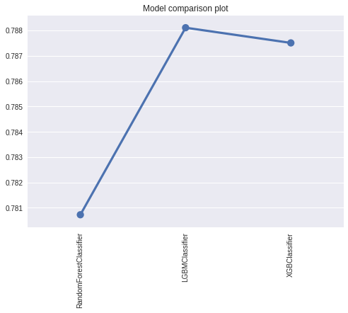
1. compare_model: This function takes as argument multiple machine learning models and returns a plot of a comparative metric. This can be used to pick a base model and also to compare models side by side. The compare model returns a tuple of the trained models and their score.

Let's demonstrate this below. We'll compare some the classification models RandomForest, LightGBM and XGBoost on the data set.

We won't be performing any advance hyperparameter tuning in this tutorial, as the goal is to show you how to use the functions and not hyperparameter tuning.

Also, you may have to install LightGbm and XGBoost before you can try out this part. Alternatively, you can use the models in scikit-learn.

from sklearn.ensemble import RandomForestClassifier
from sklearn.model_selection import train_test_split
import lightgbm as lgb
import xgboost as xgb\


#split train data into train and test set
Xtrain, Xtest, ytrain, ytest = train_test_split(train_enc, target, test_size=0.3, random_state=1)

#define models you want to compare
rf_classifier = RandomForestClassifier(n_estimators=20, max_depth=4)
lgb_classifier = lgb.LGBMClassifier(n_estimators=20, max_depth=4)
xgb_classifier = xgb.XGBClassifier(n_estimators=20, max_depth=4)

classifiers = [rf_classifier, lgb_classifier, xgb_classifier]

#compare the models
models, scores = ds.model.compare_model(models_list=classifiers, x_train=Xtrain, 
                                         y_train=ytrain, scoring_metric='accuracy')

From this sample analysis, the LGBMClassifier is currently the best model. We can make predictions with this model without retraining as shown below:

#use the best model to make prediction on the test set
pred = models[1].predict(Xtest)

get_classification_report: We can get a detailed metric report for a classification task using the get_classification_report function. This accepts as argument the predicted class and the truth value, and returns classification metrics like accuracy, f1_score, precision, recall and the confusion matrix.

ds.model.get_classification_report(pred, ytest)

Accuracy is 78.0
F1 score is 21.0
Precision is 13.0
Recall is 66.0
************************************************************************************************
confusion Matrix
             Score positive    Score negative
Actual positive 1604 445
Actual negative 34 65

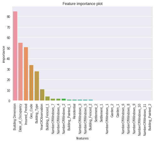
plot_feature_importance: This function can be used to make a bar plot of the most important features to a trained machine learning model.

model = models[1]  #get a model from the list of returned models
features = train_enc.columns  #get the feature names from the processed data

ds.model.plot_feature_importance(model, features)

We demonstrated the example in this tutorial using a classification task. You can also apply the same functions to your regression problems. See more here

Check the API documentation to learn more about the functions available and how to set parameters.

And we have come to the end of this tutorial. I'm sure you are eager to use datasist in your next project. This post served as a quick guide to datasist and by no means covers exclusively all functions available.

PreviousQuick Guide-Part 1 NextTutorials

Last updated 3 years ago