Quick Guide-Part 1

What is Datasist, and why should you be excited about it?

In plain English, Datasist makes data analysis, visualization, cleaning, preparation, and even modeling super easy for you during prototyping.

Because let's face it I wouldn't want to do this... (Please look at the code block below)

import pandas as pd

data = pd.read_csv('some_csv_file.csv)

missing_percent = (data.isna().sum() / data.shape[0]) * 100
cols_2_drop = missing_percent[missing_percent.values >= 80].index
df = data.drop(cols_2_drop, axis=1)  #Drop missing values

...just because I want to drop columns with missing percentage greater than or equal to 80, when I can simply do this (Please look at the beauty below)

import pandas as pd
import datasist as ds

data = pd.read_csv('some_csv_file.csv)
df = ds.drop_missing(data=data, percent=80)

**smiles, I know right, it's lazy, but damn efficient.

The goal of datasist is to abstract repetitive and mundane codes into simple, short functions and methods that can be called easily. Datasist was born out of sheer laziness, because let's face it unless you're a 100x data scientists, we all hate typing long, boring and mundane chunks of code to do the same thing repeatedly

The design of datasist is currently as of v1.5 is centered around 6 modules, namely:

1. project

2. visualization

3. feature_engineering

4. timeseries

5. model

6. structdata

This is subject to change in future versions as we are currently working on support for many other areas in the field. Check our releases or follow our social media page to stay updated.

The aim of this tutorial is to introduce you to some of the important features these modules and how you can start using them in your projects. We understand you might not like taking it all at once, so we split this tutorial into two parts.

Part 1 will cover the modules project, structdata, feature engineering, timeseries and Part 2 will cover visualization and model modules.

So without wasting more time, let's get to it.

What you will learn in this part:

• Working with the datasist structdata module.

• Feature engineering with datasist.

• Intro to visualization.

• Easy visualization with datasist.

To follow along this article, you'll need to install the datasist library. You can do that using the python pip manager. Open a terminal and run the command:

pip install datasist

Remember to use the exclamation symbol if you're running the command inside a Jupyter notebook.

!pip install datasist

Next, you need to get a dataset to work with, you can use any dataset, but for consistency, you can download the dataset we used for this tutorial here

Finally, open your Jupyter Notebook, import your libraries and dataset as shown below:

import pandas as pd
import datasist as ds  #import datasist library
import numpy as np

train_df = pd.read_csv('train_data.csv')
test_df = pd.read_csv('test_data.csv')

Working with the structdata module

The structdata module contains numerous functions for working with structured data mostly in the Pandas DataFrame format. That is, you can use the functions in this module to easily manipulate and analyze DataFrames. Let's use some of the functions available:

1. describe: We all know the describe function in Pandas, well ,we decided to extend it to support full description of a dataset at a glance.

ds.structdata.describe(train_df)

Running the command above gives the following Output:

First five data points

****	Customer Id	YearOfObservation	Insured_Period	Residential	Building_Painted	Building_Fenced	Garden	Settlement	Building Dimension	Building_Type	Date_of_Occupancy	NumberOfWindows	Geo_Code	Claim
0	H14663	2013	1.0	0	N	V	V	U	290.0	1	1960.0	.	1053	0
1	H2037	2015	1.0	0	V	N	O	R	490.0	1	1850.0	4	1053	0
2	H3802	2014	1.0	0	N	V	V	U	595.0	1	1960.0	.	1053	0
3	H3834	2013	1.0	0	V	V	V	U	2840.0	1	1960.0	.	1053	0
4	H5053	2014	1.0	0	V	N	O	R	680.0	1	1800.0	3	1053	0

Random five data points

****	Customer Id	YearOfObservation	Insured_Period	Residential	Building_Painted	Building_Fenced	Garden	Settlement	Building Dimension	Building_Type	Date_of_Occupancy	NumberOfWindows	Geo_Code	Claim
5734	H15079	2014	1.000000	0	N	V	V	U	1000.0	2	1980.0	.	83098	0
2384	H5026	2013	0.865753	1	V	V	V	U	5746.0	1	NaN	.	33096	0
6064	H1290	2014	1.000000	0	V	V	V	U	2250.0	1	1988.0	.	88383	0
4516	H13475	2013	0.580822	0	N	V	V	U	3600.0	2	1988.0	.	69294	1
6761	H4377	2013	0.580822	1	V	V	V	U	1265.0	3	NaN	.	94041	0

Last five data points

****	Customer Id	YearOfObservation	Insured_Period	Residential	Building_Painted	Building_Fenced	Garden	Settlement	Building Dimension	Building_Type	Date_of_Occupancy	NumberOfWindows	Geo_Code	Claim
7155	H5290	2012	1.000000	1	V	V	V	U	NaN	1	2001.0	.	NaN	0
7156	H5926	2013	1.000000	0	V	V	V	U	NaN	2	1980.0	.	NaN	1
7157	H6204	2016	0.038251	0	V	V	V	U	NaN	1	1992.0	.	NaN	0
7158	H6537	2013	1.000000	0	V	V	V	U	NaN	1	1972.0	.	NaN	0
7159	H7470	2014	1.000000	0	V	V	V	U	NaN	1	2004.0	.	NaN	0

Shape of data set: (7160, 14)

Size of data set: 100240

Data Types

Note: All Non-numerical features are identified as objects in pandas

	Data Type
Customer Id	object
YearOfObservation	int64
Insured_Period	float64
Residential	int64
Building_Painted	object
Building_Fenced	object
Garden	object
Settlement	object
Building Dimension	float64
Building_Type	int64
Date_of_Occupancy	float64
NumberOfWindows	object
Geo_Code	object
Claim	int64

Numerical Features in Data set

['YearOfObservation', 'Insured_Period', 'Residential', 'Building Dimension', 'Building_Type', 'Date_of_Occupancy', 'Claim']

Statistical Description of Columns

****	YearOfObservation	Insured_Period	Residential	Building Dimension	Building_Type	Date_of_Occupancy	Claim
count	7160.000000	7160.000000	7160.000000	7054.000000	7160.000000	6652.000000	7160.000000
mean	2013.669553	0.909758	0.305447	1883.727530	2.186034	1964.456404	0.228212
std	1.383769	0.239756	0.460629	2278.157745	0.940632	36.002014	0.419709
min	2012.000000	0.000000	0.000000	1.000000	1.000000	1545.000000	0.000000
25%	2012.000000	0.997268	0.000000	528.000000	2.000000	1960.000000	0.000000
50%	2013.000000	1.000000	0.000000	1083.000000	2.000000	1970.000000	0.000000
75%	2015.000000	1.000000	1.000000	2289.750000	3.000000	1980.000000	0.000000
max	2016.000000	1.000000	1.000000	20940.000000	4.000000	2016.000000	1.000000

Description of Categorical Features

****	count	unique	top	freq
Customer Id	7160	7160	H6516	1
Building_Painted	7160	2	V	5382
Building_Fenced	7160	2	N	3608
Garden	7153	2	O	3602
Settlement	7160	2	R	3610
NumberOfWindows	7160	11	.	3551
Geo_Code	7058	1307	6088	143

Categorical Features in Data set

['Customer Id', 'Building_Painted','Building_Fenced', 'Garden', 'Settlement', 'NumberOfWindows', 'Geo_Code']

Unique class Count of Categorical features

****	Feature	Unique Count
0	Customer Id	7160
1	Building_Painted	2
2	Building_Fenced	2
3	Garden	3
4	Settlement	2
5	NumberOfWindows	11
6	Geo_Code	1308

Missing Values in Data

****	features	missing_counts	missing_percent
0	Customer Id	0	0.0
1	YearOfObservation	0	0.0
2	Insured_Period	0	0.0
3	Residential	0	0.0
4	Building_Painted	0	0.0
5	Building_Fenced	0	0.0
6	Garden	7	0.1
7	Settlement	0	0.0
8	Building Dimension	106	1.5
9	Building_Type	0	0.0
10	Date_of_Occupancy	508	7.1
11	NumberOfWindows	0	0.0
12	Geo_Code	102	1.4
13	Claim	0	0.0

From the result, you can have a full description and properly understand some of the important features of your dataset at a glance, all with one line of code.

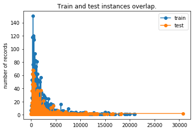
2. check_train_test_set: This function is used to check the sampling strategy of two dataset. This is important because if two dataset are not from the same distribution, then feature extraction techniques will be different as we can not extrapolate calculations from one to another.

To use this function, you must pass both dataset (train_df and test_df), a common index (customer_id) and finally any feature or column available in both dataset.

ds.structdata.check_train_test_set(train_df, test_df, index='Customer Id', col='Building Dimension')

Output:

There are 7160 training rows and 3069 test rows.

There are 14 training columns and 13 test columns.

Id field is unique.

Train and test sets have distinct Ids.

3. display_missing: You can check for the missing values in your dataset and display the result in the well formatted DataFrame.

ds.structdata.display_missing(train_df)

Output:

	features	missing_counts	missing_percent
0	Customer Id	0	0.0
1	YearOfObservation	0	0.0
2	Insured_Period	0	0.0
3	Residential	0	0.0
4	Building_Painted	0	0.0
5	Building_Fenced	0	0.0
6	Garden	7	0.1
7	Settlement	0	0.0
8	Building Dimension	106	1.5
9	Building_Type	0	0.0
10	Date_of_Occupancy	508	7.1
11	NumberOfWindows	0	0.0
12	Geo_Code	102	1.4
13	Claim	0	0.0

4. get_cat_feats and get_num_feats: Just like their names, you can use these functions to retrieve categorical and numerical features respectively as a list.

cat_feats = ds.structdata.get_cat_feats(train_df)
cat_feats

Output:

['Customer Id', 'Building_Painted', 'Building_Fenced', 'Garden', 'Settlement', 'NumberOfWindows','Geo_Code']

num_feats = ds.structdata.get_num_feats(train_df)

num_feats

Output:

['YearOfObservation','Insured_Period',Residential',BuildingDimension',Building_Type',Date_of_Occupancy','Claim']

5. get_unique_counts: Ever wanted to get the unique classes in your categorical features before you decide what encoding scheme to use? well, you can use the get_unique_count function to easily that.

ds.structdata.get_unique_counts(train_df)

Output:

	Feature	Unique Count
0	Customer Id	7160
1	Building_Painted	2
2	Building_Fenced	2
3	Garden	3
4	Settlement	2
5	NumberOfWindows	11
6	Geo_Code	1308

6. join_train_and_test: When prototyping, you may want to concatenate both train and test set, and then apply some transformations. You can use the join_train_and_test function for that. It returns a concatenated dataset, the size of the train and test data for splitting in the future

Output:

all_data, ntrain, ntest = ds.structdata.join_train_and_test(train_df, test_df)
print("New size of combined data {}".format(all_data.shape))
print("Old size of train data: {}".format(ntrain))
print("Old size of test data: {}".format(ntest))

#later splitting after transformations
train = all_data[:ntrain]
test = all_data[ntrain:]

Output:

New size of combined data (10229, 14)

Old size of train data: 7160

Old size of test data: 3069

Those are some of the popular functions in the structdata module of datasist, to see other functions and to learn more about the parameters you can tweak, check the API documentation here.

Feature engineering with datasist.

Feature engineering is the process of using data’s domain knowledge to create features that make machine learning algorithms work. It’s the act of extracting important features from raw data and transforming them into formats that are suitable for machine learning.

Some of the functions available in the feature_engineering module of datasist can help you quickly and easily perform feature engineering. Let's explore some of them below:

Functions in the feature_engineering module always returns a new and transformed DataFrame. This means, it always expects that you assign the result to a variable as nothing happens inplace.

1. drop_missing: This function drops columns/features with a specified percentage of missing values. Let's demonstrate this below:

#first let's view the percentage of missing values in the dataset
ds.structdata.display_missing(train_df)

Output:

	features	missing_counts	missing_percent
0	Customer Id	0	0.0
1	YearOfObservation	0	0.0
2	Insured_Period	0	0.0
3	Residential	0	0.0
4	Building_Painted	0	0.0
5	Building_Fenced	0	0.0
6	Garden	7	0.1
7	Settlement	0	0.0
8	Building Dimension	106	1.5
9	Building_Type	0	0.0
10	Date_of_Occupancy	508	7.1
11	NumberOfWindows	0	0.0
12	Geo_Code	102	1.4
13	Claim	0	0.0

Just for demonstration, we'll drop the column with 7.1 percent missing values.

You should not drop a column/feature with little missing values like we did above. What you should do is fill it. We do this here, for demonstration purpose only

new_train_df = ds.feature_engineering.drop_missing(train_df, percent=7.0)
ds.structdata.display_missing(new_train_df)

Output:

Dropped ['Date_of_Occupancy']

	features	missing_counts	missing_percent
0	Customer Id	0	0.0
1	YearOfObservation	0	0.0
2	Insured_Period	0	0.0
3	Residential	0	0.0
4	Building_Painted	0	0.0
5	Building_Fenced	0	0.0
6	Garden	7	0.1
7	Settlement	0	0.0
8	Building Dimension	106	1.5
9	Building_Type	0	0.0
10	NumberOfWindows	0	0.0
11	Geo_Code	102	1.4
12	Claim	0	0.0

2. drop_redundant: This function is used to remove features with no variance. That is features that contain the same class all through. We show a simple example using an artificial dataset below.

df = pd.DataFrame({'a': [1,1,1,1,1,1,1],
                  'b': [2,3,4,5,6,7,8]})

df

Output:

	a	b
0	1	2
1	1	3
2	1	4
3	1	5
4	1	6
5	1	7
6	1	8

Now, looking at the artificial dataset above, we see that column a is redundant, that is, it has the same class all through. We can drop this column automatically by passing the DataFrame to the drop_redundant function.

df = ds.feature_engineering.drop_redundant(df)
df

Output:

Dropped ['a']

	b
0	2
1	3
2	4
3	5
4	6
5	7
6	8

3. convert_dtypes: This function takes a DataFrame and automatically type-cast features that are not represented in their right types. Let's see an example using an artificial dataset as shown below:

data = {'Name':['Tom', 'nick', 'jack'],
        'Age':['20', '21', '19'], 
        'Date of Birth': ['1999-11-17','20 Sept 1998','Wed Sep 19 14:55:02 2000']}

df = pd.DataFrame(data)
df

Output:

	Name	Age	Date of Birth
0	Tom	20	1999-11-17
1	nick	21	20 Sept 1998
2	jack	19	Wed Sep 19 14:55:02 2000

Next, let's check the data types:

df.dtypes

Output:

Name object

Age object

Date of Birth object

dtype: object

The features Age and Date of Birth are suppose to be in Integer and DateTime format. By passing this DataFrame to the convert_dtype function, this can be automatically fixed.

df = ds.feature_engineering.convert_dtype(df)
df.dtypes

Output:

Name object

Age int64

Date of Birth datetime64[ns]

dtype: object

4. fill_missing_cats: As the name implies, this function takes a DataFrame, and automatically fills missing values in the categorical columns. It fills missing values using the mode of the feature. First, let's see the columns with missing values.

ds.structdata.display_missing(train_df)

Output:

	features	missing_counts	missing_percent
0	Customer Id	0	0.0
1	YearOfObservation	0	0.0
2	Insured_Period	0	0.0
3	Residential	0	0.0
4	Building_Painted	0	0.0
5	Building_Fenced	0	0.0
6	Garden	7	0.1
7	Settlement	0	0.0
8	Building Dimension	106	1.5
9	Building_Type	0	0.0
10	Date_of_Occupancy	508	7.1
11	NumberOfWindows	0	0.0
12	Geo_Code	102	1.4
13	Claim	0	0.0

From the output, we have two categorical features with missing values, the Garden and Geo_Code. Next, let's fill these features:

df = ds.feature_engineering.fill_missing_cats(train_df)
ds.structdata.display_missing(df)

Output:

	features	missing_counts	missing_percent
0	Customer Id	0	0.0
1	YearOfObservation	0	0.0
2	Insured_Period	0	0.0
3	Residential	0	0.0
4	Building_Painted	0	0.0
5	Building_Fenced	0	0.0
6	Garden	0	0.0
7	Settlement	0	0.0
8	Building Dimension	106	1.5
9	Building_Type	0	0.0
10	Date_of_Occupancy	508	7.1
11	NumberOfWindows	0	0.0
12	Geo_Code	0	0.0
13	Claim	0	0.0

5. fill_missing_nums: This is similar to the fill_missing_cats, except it works on numerical features and you can specify a fill strategy (mean, mode or median).

From the dataset, we have two numerical features with missing values, the Building Dimension and Date_of_Occupancy.

df = ds.feature_engineering.fill_missing_num(train_df)
ds.structdata.display_missing(df)

Output:

	features	missing_counts	missing_percent
0	Customer Id	0	0.0
1	YearOfObservation	0	0.0
2	Insured_Period	0	0.0
3	Residential	0	0.0
4	Building_Painted	0	0.0
5	Building_Fenced	0	0.0
6	Garden	7	0.1
7	Settlement	0	0.0
8	Building Dimension	0	0.0
9	Building_Type	0	0.0
10	Date_of_Occupancy	0	0.0
11	NumberOfWindows	0	0.0
12	Geo_Code	102	1.4
13	Claim	0	0.0

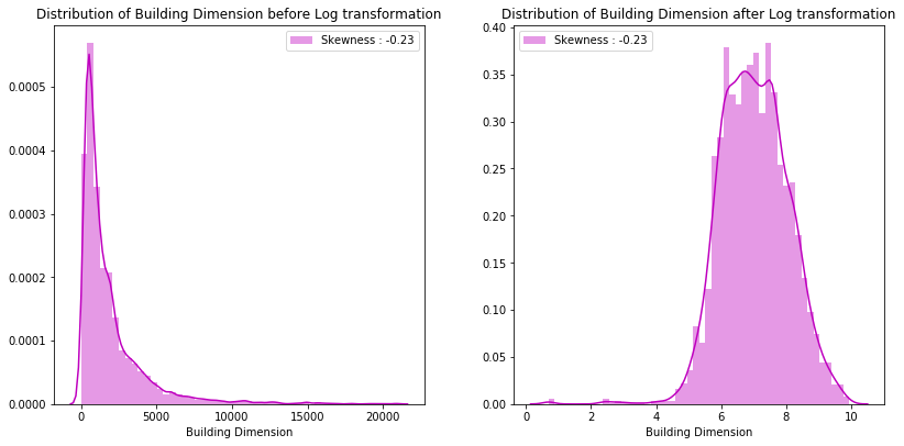
6. log_transform: This function can help you log-transform a set of features. It can also displays a before and after plot which shows the level of skewness to help you decide if log transform is effective.

After visualization of some of the data set which we will study next part, we found out that the feature Building Dimension is skewed. Let's use the log_transform function on it.

Make sure your columns do not contain missing values.

df = ds.feature_engineering.fill_missing_num(df)
df = ds.feature_engineering.log_transform(df, columns=['Building Dimension'])

7. merge_groupby: This function populates your data set with new features. These features are created by grouping your data on exisitng categorical features and calculating the aggregrate of a numerical feature present in each groups. The aggregrate function is limited to mean and count. The new feature (the aggregrated result) is then merged with the data set.

Let's illustate this by using the merge_groupby function on a new data set which is created from three columns of the orignal data set.

#sub_df is a sub data set of the orignal data set 

sub_df = df.loc[:,['Customer Id', 'Building_Type', 'Building_Fenced']]
ds.feature_engineering.merge_groupby(data = sub_df, cat_features = ['Building_Fenced'],statistics = ['count'], col_to_merge = 'Building_Type').head(5)

Output:

	Customer Id	Building_Type	Building_Fenced	Building_Fenced_Building_Type_count
0	H14663	1	V	3552
1	H2037	1	N	3608
2	H3802	1	V	3552
3	H3834	1	V	3552
4	H5053	1	N	3608

8. create_balanced_data: This function creates a balanced data set from an imbalanced one. This function is strictly used in a classification task.

Let's illustate this by using the create_balanced_data function on an artificial data set.

data = {'Name':['tom', 'nick', 'jack','remi','june', 'temi', 'ore','ayo','teni', 'tina'],
        'Age':['20', '21', '19','22','31','15','42','21','19', '20'], 
        'Sex': ['Male','Male','Female', 'Female', 'Female','Male','Female', 'Female', 'Female', 'Female']}

dfs = pd.DataFrame(data)
dfs

Output:

	Name	Age	Sex
0	tom	20	Male
1	nick	21	Male
2	jack	19	Female
3	remi	22	Female
4	june	31	Female
5	temi	15	Male
6	ore	42	Female
7	ayo	21	Female
8	teni	19	Female
9	tina	20	Female

By setting class_sizes parameter to [5,5], the function will create a new data set of exactly five records for each of the two categories Male and Female present in the target column Sex.

ds.feature_engineering.create_balanced_data (data = dfs, target = 'Sex', categories = ['Male','Female'], class_sizes = [5,5])

Output:

	Name	Age	Sex
0	tom	20	Male
1	temi	15	Male
2	ore	42	Female
3	temi	15	Male
4	ore	42	Female
5	nick	21	Male
6	remi	22	Female
7	nick	21	Male
8	june	31	Female
9	jack	19	Female

9. get_qcut: The get_qcut function cut a series into bins using the pandas qcut function and returns the resulting bins as a series with data type float for merging.

Let's illustate this by using the get_qcut function on an artificial data set.

data = {'Name':['tom', 'nick', 'jack','remi','june', 'temi', 'ore','ayo','teni', 'tina'],
        'Age':['20', '21', '19','22','31','15','42','21','19', '20'], 
        'Sex': ['Male','Male','Female', 'Female', 'Female','Male','Female', 'Female', 'Female', 'Female']}

dfs = pd.DataFrame(data)
ds.feature_engineering.get_qcut(data = dfs, col = 'Age', q = [0, .25, .5, .75, 1.] )

Output: 0 19.250 1 20.500 2 14.999 3 21.750 4 21.750 5 14.999 6 21.750 7 20.500 8 14.999 9 19.250 Name: Age, dtype: float64

0	19.250
1	20.500
2	14.999
3	21.750
4	21.750
5	14.999
6	21.750
7	20.500
8	14.999
9	19.250

Name: Age, dtype: float64

note: q is the Number of quantiles. 10 for deciles, 4 for quartiles, etc. Alternately array of quantiles, e.g. [0, .25, .5, .75, 1.] for quartiles.

To work with features like latitude and longitude, datasist has dedicated functions like bearing, manhattan_distance, get_location_center, etc, available in the feature_engineering module. You can find more details in the API documentation here.

Working with Date time features

Finally in this part, we'll talk about the timeseries module in datasist. The timeseries module contains functions for working with date time features. It can help you extract from and visualize Date Features.

1. extract_dates: This function can be used to extract specified features like day of the week, day of the year, hour, min and second of the day from a specified date feature. To demonstrate this, let's use a dataset that contains Date feature.

Get the Sendy dataset here. This dataset contains date and distance based features.

new_train = pd.read_csv("sendy_train.csv")
new_train.head(3).T

Output:

	0	1	2
Order No	Order_No_4211	Order_No_25375	Order_No_1899
User Id	User_Id_633	User_Id_2285	User_Id_265
Vehicle Type	Bike	Bike	Bike
Platform Type	3	3	3
Personal or Business	Business	Personal	Business
Placement - Day of Month	9	12	30
Placement - Weekday (Mo = 1)	5	5	2
Placement - Time	9:35:46 AM	11:16:16 AM	12:39:25 PM
Confirmation - Day of Month	9	12	30
Confirmation - Weekday (Mo = 1)	5	5	2
Confirmation - Time	9:40:10 AM	11:23:21 AM	12:42:44 PM
Arrival at Pickup - Day of Month	9	12	30
Arrival at Pickup - Weekday (Mo = 1)	5	5	2
Arrival at Pickup - Time	10:04:47 AM	11:40:22 AM	12:49:34 PM
Pickup - Day of Month	9	12	30
Pickup - Weekday (Mo = 1)	5	5	2
Pickup - Time	10:27:30 AM	11:44:09 AM	12:53:03 PM
Arrival at Destination - Day of Month	9	12	30
Arrival at Destination - Weekday (Mo = 1)	5	5	2
Arrival at Destination - Time	10:39:55 AM	12:17:22 PM	1:00:38 PM
Distance (KM)	4	16	3
Temperature	20.4	26.4	NaN
Precipitation in millimeters	NaN	NaN	NaN
Pickup Lat	-1.31775	-1.35145	-1.30828
Pickup Long	36.8304	36.8993	36.8434
Destination Lat	-1.30041	-1.295	-1.30092
Destination Long	36.8297	36.8144	36.8282
Rider Id	Rider_Id_432	Rider_Id_856	Rider_Id_155
Time from Pickup to Arrival	745	1993	455

The dataset is logistic dataset, and contains numerous Date features which we can analyze. Let's demonstrate how easy it is to extract information from the features Placement - Time and Arrival at Destination - Time using the extract_dates function.

cols = ['Placement - Time', 'Arrival at Destination - Time']
df = ds.timeseries.extract_dates(new_train, date_cols=cols)
df.head(3).T

Output:

	0	1	2
Order No	Order_No_4211	Order_No_25375	Order_No_1899
User Id	User_Id_633	User_Id_2285	User_Id_265
Vehicle Type	Bike	Bike	Bike
Platform Type	3	3	3
Personal or Business	Business	Personal	Business
Placement - Day of Month	9	12	30
Placement - Weekday (Mo = 1)	5	5	2
Confirmation - Day of Month	9	12	30
Confirmation - Weekday (Mo = 1)	5	5	2
Confirmation - Time	9:40:10 AM	11:23:21 AM	12:42:44 PM
Arrival at Pickup - Day of Month	9	12	30
Arrival at Pickup - Weekday (Mo = 1)	5	5	2
Arrival at Pickup - Time	10:04:47 AM	11:40:22 AM	12:49:34 PM
Pickup - Day of Month	9	12	30
Pickup - Weekday (Mo = 1)	5	5	2
Pickup - Time	10:27:30 AM	11:44:09 AM	12:53:03 PM
Arrival at Destination - Day of Month	9	12	30
Arrival at Destination - Weekday (Mo = 1)	5	5	2
Distance (KM)	4	16	3
Temperature	20.4	26.4	NaN
Precipitation in millimeters	NaN	NaN	NaN
Pickup Lat	-1.31775	-1.35145	-1.30828
Pickup Long	36.8304	36.8993	36.8434
Destination Lat	-1.30041	-1.295	-1.30092
Destination Long	36.8297	36.8144	36.8282
Rider Id	Rider_Id_432	Rider_Id_856	Rider_Id_155
Time from Pickup to Arrival	745	1993	455
Placement - Time_dow	Sunday	Sunday	Sunday
Placement - Time_doy	335	335	335
Placement - Time_dom	1	1	1
Placement - Time_hr	9	11	12
Placement - Time_min	35	16	39
Placement - Time_is_wkd	0	0	0
Placement - Time_yr	2019	2019	2019
Placement - Time_qtr	4	4	4
Placement - Time_mth	12	12	12
Arrival at Destination - Time_dow	Sunday	Sunday	Sunday
Arrival at Destination - Time_doy	335	335	335
Arrival at Destination - Time_dom	1	1	1
Arrival at Destination - Time_hr	10	12	13
Arrival at Destination - Time_min	39	17	0
Arrival at Destination - Time_is_wkd	0	0	0
Arrival at Destination - Time_yr	2019	2019	2019
Arrival at Destination - Time_qtr	4	4	4
Arrival at Destination - Time_mth	12	12	12

You can specify the features to return by changing the subset parameter. For instance, we could specify that we only want day of the week and hour as shown below

cols = ['Placement - Time', 'Arrival at Destination - Time']
df = ds.timeseries.extract_dates(new_train, date_cols=cols, subset=['dow', 'hr'])
df.head(3).T

Output:

	0	1	2
Order No	Order_No_4211	Order_No_25375	Order_No_1899
User Id	User_Id_633	User_Id_2285	User_Id_265
Vehicle Type	Bike	Bike	Bike
Platform Type	3	3	3
Personal or Business	Business	Personal	Business
Placement - Day of Month	9	12	30
Placement - Weekday (Mo = 1)	5	5	2
Confirmation - Day of Month	9	12	30
Confirmation - Weekday (Mo = 1)	5	5	2
Confirmation - Time	9:40:10 AM	11:23:21 AM	12:42:44 PM
Arrival at Pickup - Day of Month	9	12	30
Arrival at Pickup - Weekday (Mo = 1)	5	5	2
Arrival at Pickup - Time	10:04:47 AM	11:40:22 AM	12:49:34 PM
Pickup - Day of Month	9	12	30
Pickup - Weekday (Mo = 1)	5	5	2
Pickup - Time	10:27:30 AM	11:44:09 AM	12:53:03 PM
Arrival at Destination - Day of Month	9	12	30
Arrival at Destination - Weekday (Mo = 1)	5	5	2
Distance (KM)	4	16	3
Temperature	20.4	26.4	NaN
Precipitation in millimeters	NaN	NaN	NaN
Pickup Lat	-1.31775	-1.35145	-1.30828
Pickup Long	36.8304	36.8993	36.8434
Destination Lat	-1.30041	-1.295	-1.30092
Destination Long	36.8297	36.8144	36.8282
Rider Id	Rider_Id_432	Rider_Id_856	Rider_Id_155
Time from Pickup to Arrival	745	1993	455
Placement - Time_dow	Sunday	Sunday	Sunday
Placement - Time_hr	9	11	12
Arrival at Destination - Time_dow	Sunday	Sunday	Sunday
Arrival at Destination - Time_hr	10	12	13

****

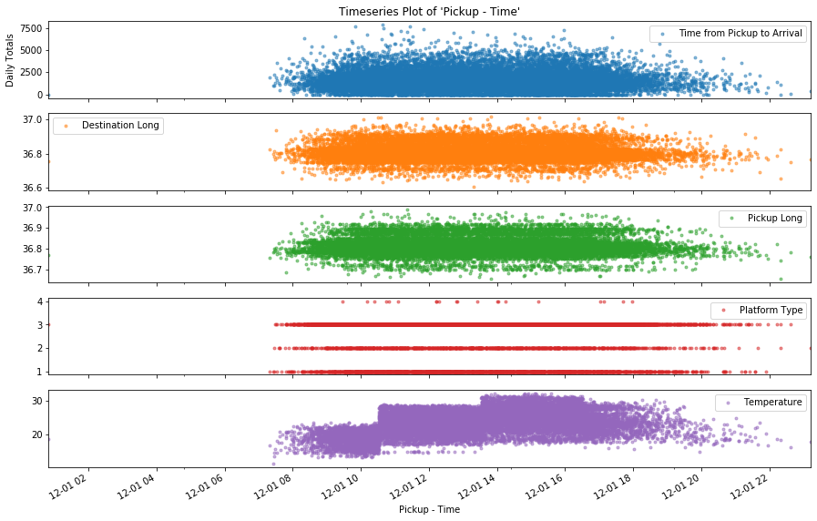
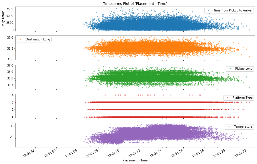
2. timeplot: The timeplot function can help you visualize a set features against a particular time feature. This can help you identify trends and patterns. To use this function, you can pass a set of numerical cols, and then specify the Date feature you want to plot against. We demonstrate this below by plotting the numerical features Time from Pickup to Arrival, Destination Long, Pickup Long and Platform Type, Temperature against the time feature Placement-Time

num_cols = ['Time from Pickup to Arrival', 'Destination Long', 'Pickup Long','Platform Type', 'Temperature']
ds.timeseries.timeplot(new_train, num_cols=num_cols,
                       time_col='Placement - Time')

Next, let's change the time feature to Pickup-Time:

num_cols = ['Time from Pickup to Arrival', 'Destination Long', 'Pickup Long','Platform Type', 'Temperature']
ds.timeseries.timeplot(new_train, num_cols=num_cols,
                       time_col='Pickup - Time')

And with that, we have come to the end of this section of the tutorial. To learn more about datasist and other functions available, be sure to check the API documentation here.

In Part 2, we will cover the visualization, model and project module.